What is a positive ELISpot response?
Published: October 14, 2022
Updated: June 26, 2023
6 minute read
Authored by: Jens Gertow
When analyzing your spot numbers, it’s not always obvious whether there is a true difference between the negative control and the spots of the antigen-stimulated wells. In this guide, we describe a non-parametric statistical test for determining positive responses.
It’s tempting to look at ELISpot or FluoroSpot results, subtract the background spots and then consider all spots above this level as a positive response. But let’s consider a result where 10 background spots are subtracted from 300 antigen-specific spots – and compare that to 200 background spots being subtracted from 490 antigen-specific spots. Both examples generate the same difference of 290 spots, but we’d argue that the first example shows a stronger case of induced immunity.
Empirical approaches are limited
The example above describes an empirical approach. In such a methodology, the researcher typically decide on an absolute difference (“at least 10 spots more”) and/or x-fold difference (“2.5 times the spots in background”) between the antigen-stimulated experimental wells and the negative control wells. However, cellular assays are inherently complex, as every replicate essentially contains its own living cell culture, and you therefore might have quite variable spot counts in replicates. This limits the analysis, as mean responses from highly variable replicates gives less-convincing evidence of a positive response than the means derived from replicates with low variability, although the empirical rule might say that both should be considered positive responses.
Use a statistical method instead: DFR
In general, a statistical method is performed by constructing a null hypothesis and an alternative hypothesis and then using the data to test the evidence against the null hypothesis. As one cannot assume normal distribution of spot numbers in the limited number of replicates usually employed in ELISpot/FluoroSpot, a non-parametric statistical test is a more suitable choice than for example the commonly used statistical T-test. For ELISpot and FluoroSpot, we recommend a non-parametric test called the distribution-free resampling (DFR), or its stricter variant, the DFR(2x):
- DFR: The null hypothesis is that the mean of the experimental well is less than or equal to the mean of the negative control wells; the alternative is that it exceeds this.
- DFR(2x): The null hypothesis is that the mean of the experimental well is less than or equal to twice the mean of the negative control wells; the alternative is that it exceeds this.
DFR or DFR(2x) – it's your choice
The difference between DFR and DFR(2x) is (not exactly – but a bit) like choosing between a level of significance of 0.05 and 0.01. In most cases, like if you have stimulated T cells with a peptide pool and are looking for low to moderate cytokine responses regardless of background, the DFR is perfectly adequate. Choose DFR(2x) only when you need really stringent control over false positives, for example when you are not expecting a response (e.g., if you stimulate with CD8 peptides and then look for Th2 cytokines instead of the expected Th1 cytokines).
Planning your experiment
Both DFR methods require a minimum number of replicates to ensure adequate power: at least three replicates for experimental and negative control wells. This doesn’t only make sense in terms of statistical power, but also for how much you can trust your data, regardless if you choose the DFR method or not. Let’s say you run only duplicates and get 13 spots in one well and 120 spots in the other well – you will have no idea which one is more correct. But if you are running in triplicates and see 13 spots, 120 spots and 110 spots, then you can suspect that something has gone wrong in the 13 spot-well, and either treat it as an outlier or re-run the sample.
How to calculate DFR and DFR(2x)
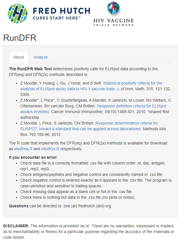
The procedure of calculating DFR is not trivial, but luckily, the primary author Dr. Zoe Moodie at Fred Hutch has published a free-to-use web tool doing these calculations for you. All you have to do is arrange the experiment with the suitable number of replicates. Please follow our step-by-step guide below:
1. Open the link RunDFR (rundfr.fredhutch.org)
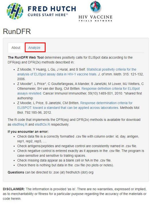
2. Click the Analyze tab
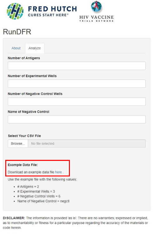
3. Download the example file (example.csv)
4. Open the downloaded file in Excel.
- Column A, “id”, represents sample ID:s, e.g., the different donors.
- Column C, “antigen”, represents stimulation conditions and negative control (unstimulated cells).
- Columns D-I, “a1, a2, a3, a4, a5, and a6”, represent your replicates and shows the different spot numbers.
- To use DFR and DFR(2x), you need to run the samples in at least triplicates (a1, a2, a3).
5. Overwrite the existing data in the example file with your own data. Add/remove/change antigens, add replicates and donors, change names of the negative control – whatever your experiment needs.
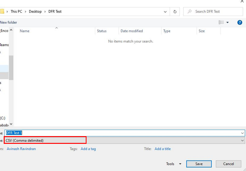
6. Save the file as .csv, not .xlsx. If you see multiple CSV options, choose the option CSV (Comma delimited).
7. Go to the Analyze tab of RunDFR (rundfr.fredhutch.org) again.
8. Fill in:
- Number of Antigens = number of different stimulation conditions (2 in the example file, “tyr” and “flu”). NB! Do not count negative control as an antigen.
- Number of Experimental Wells = number of replicates of your sample wells (3 in the example file)
- Number of Negative Control Wells = number replicates of your negative control (6 in the example file)
- Name of Negative Control, which is “negctl” in the example file, but might be “unstim” or something similar in your own experiment. Just make sure you write it exactly as it is written in the .csv-file
9. Upload your .csv file by pressing Browse, find it, and then press open (NB! You must fill in the fields in step 8 before uploading the file, otherwise you will get an error message).
10. Ta-da! Now you should see your results to the right. Columns a1, a2, a3,… are the replicates of your sample wells whereas c1, c2, c3,… signify the replicates of the negative controls. The column showing results for DFR is called “DFR(eq) response”, and the column showing DFR(2x) is called “DFR(2x) response”. A “1.00” means that the null hypothesis has been discarded, meaning the experimental wells are not equal to the negative control, meaning you are detecting a positive response. A “0.00” means that there was no difference between the experimental well and the negative control.
Read more on the development and details of DFR and DFR(2x):
- Moodie et al., Response determination criteria for ELISPOT: toward a standard that can be applied across laboratories. Methods Mol Biol. 2012
- Moodie et al., Response definition criteria for ELISpot assays revisited. Cancer Immunol Immunother 2010
Please make sure to cite the two papers above if you choose to publish data where the DFR methodology has been used.
Statistics is one thing, but other variables at the laboratory level also need to be minimized to ensure the sturdiness of the collected data – please follow our Step-by-step guides to ELISpot or FluoroSpot to optimize your lab work.


